Simulate fluid mechanics with MPI
You can find this tutorial in the demos folder of your Jupyter notebook environment.
- athena_read.py
- athinput.orszag-tang
- fluid_dynamics_mpi.ipynb
- plot_output.py
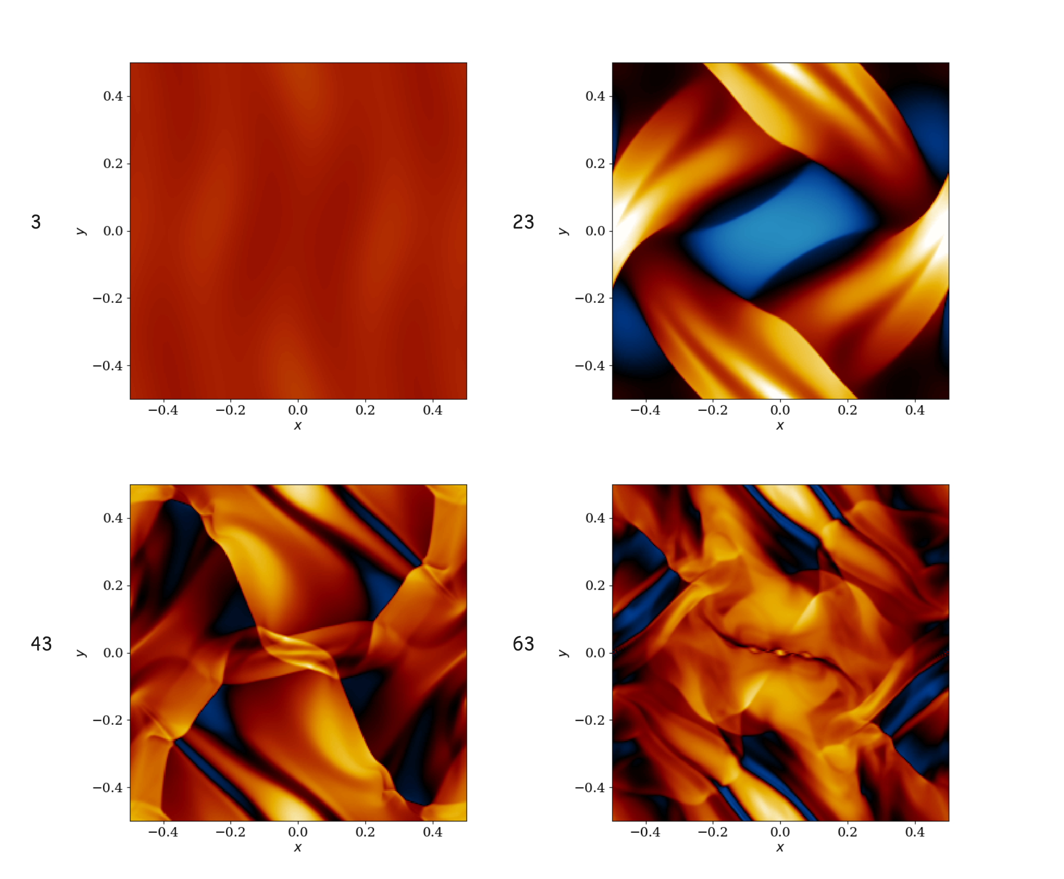
frames 3, 23, 43, and 63 of a simulation of the Orszag-Tang vortex. Scroll to the end for a video
This tutorial demonstrates a simulation and visualization of a well-known problem in magnetohydrodynamics.
The simulation is parallelized using the Camber mpi package, and it uses the Athena library to execute Athena++ code on Camber’s OpenMPI infrastructure.
Simulate a 2D Orszag-Tang vortex
The following steps create an MPI cluster to compute the Orszag-Tang Vortex, a popular demonstration problem in fluid mechanics. After the output is generated, an imported Python script creates a visualization.
Spin-Up MPI cluster
The first step is to import Camber and initialize the MPI cluster:
import camber# download Athena++ from public repo if not already present in your directory
!git clone https://github.com/PrincetonUniversity/athena.gitNow create an MPI job to compile Athena++.
This step ensures the code compiles with the correct MPI environment:
# Now we create an MPI job to compile Athena++. This step ensure the code is compiled with the correct MPI environment
compile_job = camber.mpi.create_job(
    command="cd athena && python configure.py -b --prob=orszag_tang -mpi -hdf5 --hdf5_path=${HDF5_HOME} && make clean && make all -j$(nproc)",
    engine_size="SMALL"
)
Check the compile_job output to monitor the job status:
compile_jobOnce the job status turns to COMPLETED, use read_logs to check the output:
compile_job.read_logs(tail_lines=10)If you want to peruse the compile logs in more detail, you can also download the log file with download_log.
You can open the log file directly in your jupyter notebook and check its contents.
compile_job.download_log()Run the MPI job
After compilation finishes, use the create_job method to start the Orszag-Tang simulation using the Athena binary and input file:
# run camber with a medium instance
run_job = camber.mpi.create_job(
    command="mpirun -np 16 athena/bin/athena -i athinput.orszag-tang",
    engine_size="MEDIUM"
)
# check job status
run_job# Check the job progress once it begins running or has completed
run_job.read_logs(tail_lines=10)Once the job starts running, Camber generates a number of OrszagTang output files. This output serves as the input for visualization in the next section.
When the job finishes, you can capture the output with download_log.
run_job.download_log()To view these logs, check the folder where you are running this workload for a file called job_<JOB_ID>.log
Read and visualize output
Now use a plot function generate images for your output.
First, if it doesn’t exist, create a file for your output images:
!mkdir output_imagesNow import the plot function from your local files and run it on your input.
This generates 100 PNG files in your output_images directory:
# import a custom script for reading and plotting the hdf5 outputs, placing images in the output_images directory
from plot_output import plot_output
plot_output()
Turn the images into a video
The plot_output function from the preceding step also generates a movie from all the output images. Here is a 2D simulation of the Orszag-Tang Vortex:
from IPython.display import Video
Video("density.mov")Read more
For more fluid dynamics and MPI, try the notebook Parallel Athena simulations on MPI.