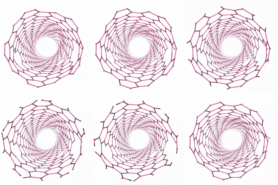
Carbon Nanotube Dynamics
You can find this application in the demos folder of your Jupyter notebook environment.
- 📝 lammps.ipynb
- 📝 sim.gif
- 📝 unbreakable.data
- 📝 unbreakable.inc
- 📝 unbreakable.lmp
LAMMPS Molecular Dynamics Simulation
This tutorial demonstrates how to run a LAMMPS (Large-scale Atomic/Molecular Massively Parallel Simulator) molecular dynamics simulation using Camber. LAMMPS is a powerful tool for simulating the dynamics of atoms and molecules, commonly used for studying materials science, chemistry, and biological systems.
In this example, we’ll simulate a carbon nanotube structure using the “unbreakable” simulation setup, which demonstrates molecular dynamics of a complex carbon structure. The workflow includes:
- Setting up and running the LAMMPS simulation
- Creating interactive visualizations of the trajectory output
Import Camber Package
First, we import the Camber package which provides the interface for running LAMMPS simulations on the cloud platform:
import camberConfigure and Submit LAMMPS Job
Here we configure and submit a LAMMPS molecular dynamics job:
command="lmp -in unbreakable.lmp": Specifies the LAMMPS command to execute the input scriptnode_size="XSMALL": Indicates the node size for the simulationwith_gpu=False: Runs the simulation on CPU (set to True for GPU acceleration)
The simulation uses these input files:
unbreakable.lmp: Main LAMMPS input script defining the simulation parametersunbreakable.data: Initial molecular structure data for the carbon nanotubeunbreakable.inc: Include file with additional force field parameters
lmp_job = camber.lammps.create_job(
    command="lmp -in unbreakable.lmp",
    node_size="XSMALL",
    with_gpu=False
)
Check Job Status
Monitor the job status to track the simulation progress:
lmp_job.statusMonitor Job Execution
To monitor job execution in real-time, use the read_logs() method to view the LAMMPS output and simulation progress (please, stand by patiently until the output appears):
lmp_job.read_logs()Analyze and Visualize Trajectory
Once the LAMMPS simulation is complete, we can analyze and visualize the molecular dynamics trajectory. This section:
- Loads the trajectory: Uses MDAnalysis to read the LAMMPS trajectory file (
trajectory.lammpstrj) - Processes molecular bonds: Attempts to identify chemical bonds between atoms for better visualization
- Creates interactive visualization: Uses NGLView to display the molecular structure with playback controls
- Adds user controls: Provides play/pause and frame slider widgets for exploring the dynamics
The visualization shows the time evolution of the carbon nanotube structure during the molecular dynamics simulation:
import os
import MDAnalysis as mda
import nglview as nv
import ipywidgets as widgets
from IPython.display import display
import numpy as np

base_path = os.getcwd()
u = mda.Universe(os.path.join(base_path, "trajectory.lammpstrj"), format="LAMMPSDUMP")

try:
    from MDAnalysis.lib.distances import distance_array
    positions = u.atoms.positions
    distances = distance_array(positions, positions)
    bond_pairs = [(i, j) for i in range(len(u.atoms)) for j in range(i+1, len(u.atoms)) if 1.2 <= distances[i, j] <= 1.8]
    if bond_pairs:
        u.add_TopologyAttr('bonds', np.array(bond_pairs))
except:
    try:
        u.atoms.guess_bonds(vdwradii={'1': 2.0}, fudge_factor=0.8)
    except:
        pass

view = nv.show_mdanalysis(u, step=1)
view.clear_representations()

try:
    if len(u.bonds) > 0:
        view.add_representation('ball+stick', selection='all', radius=0.05, bond_radius=0.05, color='hotpink')
    else:
        raise ValueError()
except:
    view.add_representation('licorice', selection='all', radius=0.1, color='hotpink')

play = widgets.Play(value=0, min=0, max=u.trajectory.n_frames-1, step=1, interval=10, description="▶️")
frame_slider = widgets.IntSlider(value=0, min=0, max=u.trajectory.n_frames-1, step=1, description='Frame:')

widgets.jslink((play, 'value'), (view, 'frame'))
widgets.jslink((frame_slider, 'value'), (view, 'frame'))

display(widgets.HBox([play, frame_slider]))
view