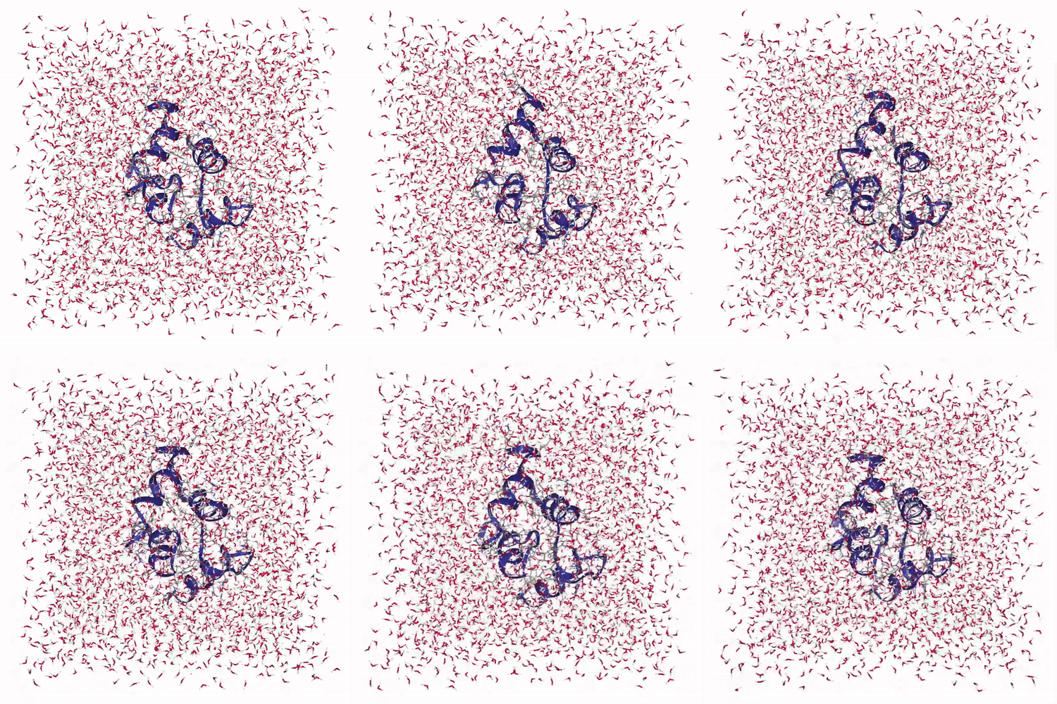
Protein in Electrolyte
You can find this application in the demos folder of your Jupyter notebook environment.
- 📝 1cta.pdb
- 📝 gromacs.ipynb
- 📝 sim.gif
- 📝 sim.sh
- 📝 topol.top
- 📝 minimize.mdp
- 📝 npt.mdp
- 📝 nvt.mdp
GROMACS Molecular Dynamics Simulation
This tutorial demonstrates how to run a GROMACS (GROningen MAchine for Chemical Simulations) molecular dynamics simulation using Camber. GROMACS is one of the most widely used molecular dynamics packages, particularly popular for studying biomolecular systems like proteins, lipids, and nucleic acids.
In this example, we’ll simulate a protein in electrolyte solution using a comprehensive workflow that includes:
- Energy minimization to remove bad contacts
- NVT equilibration to establish proper temperature
- Interactive visualization of the simulation trajectory
Import Camber Package
First, we import the Camber package which provides the interface for running GROMACS simulations on the cloud platform:
import camberConfigure and Submit GROMACS Job
Here we configure and submit a GROMACS molecular dynamics job:
command="sh ./sim.sh": Executes the simulation script that runs the complete GROMACS workflownode_size="XSMALL": Indicates the node size for the simulationwith_gpu=True: Enables GPU acceleration for faster molecular dynamics calculations
The simulation uses these input files:
sim.sh: Shell script orchestrating the complete GROMACS workflow1cta.pdb: Initial protein structure (Protein Data Bank format)topol.top: Molecular topology file defining atoms, bonds, and force field parametersinputs/: Directory containing molecular dynamics parameter files:minimize.mdp: Energy minimization parametersnvt.mdp: NVT (constant volume/temperature) equilibration parametersnpt.mdp: NPT (constant pressure/temperature) production parameters
gmx_job = camber.gromacs.create_job(
    command="sh ./sim.sh",
    node_size="XSMALL",
    with_gpu=True
)
Check Job Status
Monitor the job status to track the simulation progress through the multi-step GROMACS workflow:
gmx_job.statusMonitor Job Execution
To monitor job execution in real-time, use the read_logs() method to view the GROMACS output, including energy minimization progress, equilibration statistics, and production run details:
gmx_job.read_logs()Analyze and Visualize Trajectory
Once the GROMACS simulation is complete, we can analyze and visualize the molecular dynamics trajectory. This section:
Loads the trajectory: Uses MDAnalysis to read the GROMACS trajectory files:
min-s.tpr: Processed structure file containing topology and coordinatesnvt_nopbc.xtc: Trajectory file with periodic boundary conditions removed
Creates interactive visualization: Uses NGLView to display the protein structure with:
cartoonrepresentation for the protein backbonelicoricerepresentation for solvent molecules (SOL)- Adjustable frame stepping for smooth playback
Adds playback controls: Provides a play widget with customizable speed for exploring the protein dynamics over time
The visualization shows how the protein structure evolves during the molecular dynamics simulation, including conformational changes and solvent interactions:
import os
import MDAnalysis as mda
import nglview as nv
import ipywidgets as widgets
from IPython.display import display

# 1) load your PBC-corrected trajectory
base_path = os.getcwd()
u = mda.Universe(
    os.path.join(base_path, "output/min-s.tpr"),
    os.path.join(base_path, "output/nvt_nopbc.xtc")
)
view = nv.show_mdanalysis(u, step=10)

view.clear_representations()
view.add_representation('cartoon', selection='protein')
view.add_representation('licorice', selection='resname SOL', radius=0.1)

# 2) make a Play widget to drive `view.frame`
play = widgets.Play(
    value=0,
    min=0,
    max=view.max_frame,
    step=1,
    interval=10,      # ms between frames; lower = faster
    description="▶️",
    continuous_update=True
)

# 3) link play.value → view.frame
widgets.jslink((play, 'value'), (view, 'frame'))

# 4) display controls + viewer
display(widgets.HBox([play]))
view